Chapter 5 Simple Linear Regression
The first analysis that we will go over is the simple linear regression. Typically, this is one of the last analyses that is taught in introductory statistics in psychology; however, we will go over the simple linear regression first because its steps are essentially identical to the GLM (i.e., OLS regression) and provides a foundation for the GLM framework.
The simple linear regression is typically taught to be used in understanding the relationship between two continuous variables, especially if one can predict the other.
However, the simple linear regression is a specific case of regression 2 where variables can actually be either continuous or categorical, the number of predictor variables can be more than one, and causation is not a requirement. Thus, regression is applicable to most data types.
The simple linear regression is written as:
\[Y = \beta_0 + \beta_1X + \varepsilon\]
where \(Y\) is the dependent (or response) variable, \(\beta_0\) is the intercept, \(\beta_1\) is the slope, \(X\) is the independent (or predictor) variable, and \(\varepsilon\) is the error.
We will use the terms dependent variable (DV) and response variable interchangeably throughout the book. We will also use the terms independent variable (IV) or predictor variable interchangeably.
\(\beta\) represents the true population value, while \(b\) represents the unstandardized estimate of the true population value that we will obtain from our analysis. For example, \(\beta_1\) represents the true population slope, while \(b_1\) represents the unstandardized estimate of the true population slope (or sample).
Thus, a predicted model (as opposed to the above true hypothesized model) would be written as:
\[\hat{Y} = b_0 + b_1X\]
where \(\hat{Y}\) represents the predicted dependent (or response) variable.
Both equations should look familiar to the slope-intercept form learned in algebra:
\[y = mx + b\]
where \(b\) is the intercept, and \(m\) is the slope.
The intercept and slope have the same meaning as they did in algebra. The intercept represents the value of \(Y\) when \(X\) is 0, and the slope represents the change in \(Y\) (\(\Delta Y\)) over the change in \(X\) (\(\Delta X\)). In other words, the intercept represents the value of the DV when the IV is 0, and the slope represents the change in the DV over the change in the IV.
Note that the \(b\) in the slope-intercept form is not the same and should not be confused with the \(b\) in the simple linear regression. The \(b\) in the simple linear regression is the slope, while the \(b\) in the slope-intercept form is the intercept. Unfortunately, using the same symbol for different terms and using different symbols for the same term is prevalent in statistics.
For a practical example of the simple linear regression, let’s say that we were interested in examining if there is a relationship between the amount of years since a professor has earned their Ph.D. and their salary.
For this example, we will use the datasetSalaries dataset.
5.1 Null and research hypotheses
\[Model: Salary = \beta_0 + \beta_1 YearsSincePhD + \varepsilon\] \[H_0: \beta_1 = 0\] \[H_1: \beta_1 \ne 0\]
where \(\beta_0\) is the intercept, \(\beta_1\) is the slope, \(H_0\) is the null hypothesis and \(H_1\) is the research or alternative hypothesis. Typically, the model is written as the hypothesized true model and thus the use of \(\beta\) rather than \(b\).
In this example, the null hypothesis states that the slope is equal to 0, or that there is no relationship between \(X\) (years since a professor has earned their Ph.D.) and \(Y\) (their 9-month academic salary). (Note: The null hypothesis is sometimes referred to as the nil hypothesis in psychology since we are typically comparing our estimate against 0, or nil).
The research hypothesis states that the slope is not equal to 0, or that there is a relationship between \(X\) (years since a professor has earned their Ph.D.) and \(Y\) (their 9-month academic salary).
The model, null hypothesis, and research hypothesis are identical for both traditional and GLM approaches.
The intercept can also be tested and its null and research hypotheses are: \[H_0: \beta_0 = 0\] \[H_1: \beta_0 \ne 0\]
The null hypothesis states that the intercept is equal to 0. In other words, the value of \(Y\) (9-month academic salary) when \(X\) (years since a professor has earned their Ph.D.) is 0 is not different than 0 ($0). (Note: Zero represents professors who have just earned their Ph.D. up to those who have earned their Ph.D. for less than a year because yrs.since.phd was collected as integers and anything less than a year would be coded as 0.)
The research hypothesis states that the intercept is not equal to 0. In other words, the value of \(Y\) (9-month academic salary) when \(X\) (years since a professor has earned their Ph.D.) is 0 is different than 0 ($0)
Again, the null and research hypotheses are identical for both traditional and GLM approaches.
5.2 Statistical analyses
To perform the simple linear regression in R, we can use the lm() function.
The first input is the formula of the model, which is the DV, followed by a tilde sign (~), followed by the IV. (Note: 1 is a placeholder for the intercept. The same analysis with identical results can be obtained without the 1. However, we place 1 there to remind us that 1 represents the intercept to gain intuition of the formula).
In our case, the DV of salary is be the first variable, followed by a ~ and the IV of yrs.since.phd. Notice the similarity between the model and formula. The second input is the dataset (i.e., datasetSalaries).
We will save the analysis into an object named model. model can be any name and was chosen for simplicity.
We can obtain the ANOVA source table by using the Anova function within the cars package.
## Anova Table (Type III tests)
##
## Response: salary
##                   Sum Sq  Df  F value    Pr(>F)
## (Intercept)   8.3369e+11   1 1099.706 < 2.2e-16 ***
## yrs.since.phd 6.3852e+10   1   84.226 < 2.2e-16 ***
## Residuals     2.9945e+11 395
## ---
## Signif. codes:  0 '***' 0.001 '**' 0.01 '*' 0.05 '.' 0.1 ' ' 1
Note: We prefer the Anova function with a capitol A over the anova function with a lowercase a because we can specify the type of sum of squares. Breifly, The sum of squares in the anova function is type I sums of squares and cannot be changed while we can specify type III sums of squares, which is the default among most statistical softwares, using the Anova function. To learn more about different types of sum of squares, check out Mangiafico’s explanation.
5.2.1 How do we read the ANOVA source table?
We can look at the variable of interest in the first column and read across that particular variable’s row for its statistical information.
For example, let’s first examine the statistics associated with the variable (Intercept). The sums of squares (Sum Sq, which is also abbreviated as \(SS\)) associated with the (Intercept) is 8.37e+11, the degrees of freedom (Df, specifically, degrees of freedom reduced) is 1, the F-statistic (F value) is 1099.71, and the p-value (Pr>F) is < 2.2e-16.
The F value or F-statistic conceptually provides a ratio of explained to unexplained variability. Explained variability is how much the DV can be explained by IVs while unexplained variability is how much variability is not explained by the IV.
The mathematical formula of the F-statistic can conceptually be thought of as:
\[F = \frac{explained\ variability}{unexplained\ variability}\]
Thus, if the IV can’t explain any of the variability within the DV, then the F-statistic is less than or equal to 1.
However, if the IV(s) can explain the DV, the F-statistic will be larger than 1. In other words, the higher the F-statistic, the more the IV(s) explain(s) the variability in the DV compared to its inability to explain the DV.
Thus, the interpretation of the F-statistic of the (Intercept) is that the (Intercept) can explain the variability in salary 1099.71 times more than the (Intercept)’s inability to explain the variability in salary. 3
The Pr(>F) or p-value associated with the Intercept is < 2.2e-16. The p-value is the probability of obtaining that particular F-statistic or more extreme assuming that the null hypothesis is true. In other words, the probability of obtaining this F-statistic by chance is extremely small.
Since yrs.since.phd was our main predictor of interest (and for extra practice), let’s also look at the statistics associated with yrs.since.phd.
The F-statistic associated with yrs.since.phd is 84.23, and can be interpreted as yrs.since.phd explains the variability in salary 84.23 times more than years.since.phd’s inability to expain the variability in salary. 4.
The p-value associated with yrs.since.phd is also < 2.2e-16 with identical interpretations for the p-value of the (Intercept).
We can also obtain the coefficients table by using the summary() function.
##
## Call:
## lm(formula = salary ~ 1 + yrs.since.phd, data = datasetSalaries)
##
## Residuals:
##    Min     1Q Median     3Q    Max
## -84171 -19432  -2858  16086 102383
##
## Coefficients:
##               Estimate Std. Error t value Pr(>|t|)
## (Intercept)    91718.7     2765.8  33.162   <2e-16 ***
## yrs.since.phd    985.3      107.4   9.177   <2e-16 ***
## ---
## Signif. codes:  0 '***' 0.001 '**' 0.01 '*' 0.05 '.' 0.1 ' ' 1
##
## Residual standard error: 27530 on 395 degrees of freedom
## Multiple R-squared:  0.1758, Adjusted R-squared:  0.1737
## F-statistic: 84.23 on 1 and 395 DF,  p-value: < 2.2e-16
5.2.2 How do we read the coefficients table?
Similarly, we can look at the variable of interest in the first column and read across that particular variable’s row for its statistical information.
Again, let’s first take a look at the statistics associated with the (Intercept). The Estimate of the (Intercept) is 91718.7, the standard error (Std. Error) is 2765.8, the t-statistic (t value) is 33.162, and the p-value ((Pr>|t|)) is < 2e-16.
The Estimate of the (Intercept) is the predicted intercept value, \(b_0 = 91718.7\). Thus, the predicted salary when \(yrs.since.phd = 0\) is $91,718.70. In other words, when a professor has had their Ph.D. for less than a year, their salary is predicted to be $91,718.70.
The t value or t-statistic is similar to the F-statistic, and can also be conceptually thought of as the ratio of explained variability to unexplained variability. The t-statistic is equal to the square root of the F-statistic when the degrees of freedom is 1 5 6. Thus, the t-statistic interpretation is that the (Intercept) explains the variability in salary 33.162 times more than its inability to explain salary.
The p-value or Pr(>|t|) of <2e-16 is the probability of obtaining that particular t-statistic or a value more extreme than the t-statistic assuming that the null hypothesis is true, which is the same value from the ANOVA source table.
Let’s also examine statistics for yrs.since.phd. The Estimate of yrs.since.phd is 985.3, the Std. Error is 107.4, the t value is 9.18, and the Pr(>|t|) is <2e-16.
The Estimate of the yrs.since.phd is the estimated slope, \(b_1 = 985.3\). Thus, salary is predicted to change by $985.30 for every 1 unit increase in yrs.since.phd 7. In other words, salary is predicted to increase by $985.30 for every additional year a professor has earned their Ph.D.
The t-statistic can be interpreted as yrs.since.phd explains the variability in salary 9.18 times more than yrs.since.phd’s inability to the explain the variability in salary.
The p-value of yrs.since.phd is identical to the p-value of the (Intercept) and has identical interpretations.
Now, if wanted, we can fill in our predicted model, \(\hat{Y} = b_0 + b_1X\), with the estimates from the coefficients table to predict (or estimate) other values of salary given a certain number of years since a professor has earned their Ph.D.
\[\hat{salary} = b_0 + b_1*yrs.since.phd = 91718.7+985.3*yrs.since.phd\]
For example, let’s say that we were interested in estimating the salary of professor’s who have worked for 2 years.
\[\hat{salary} = 91718.7+985.3*yrs.since.phd = 91718.7+985.3*2 = 93689.3\]
5.3 Statistical decision
To determine if yrs.since.phd is statistically significant in predicting salary, we will compare its p-value with the alpha level (\(\alpha\)) of 0.05. \(\alpha\) is the Type I error rate, or the probability that we are incorrectly rejecting the null hypothesis when it is actually true.
Given that the p-value of <2.2e-16 for the yrs.since.phd is less than the alpha level (\(\alpha\)) of 0.05, we will reject the null hypothesis.
We can also determine if the intercept is statistically significant. Given, that the (Intercept) had an identical p-value, we will also reject the null hypothesis.
5.4 APA statement
A regression was performed to test if the amount of years since obtaining a Ph.D. was related to their salary. The amount of years since obtaining a Ph.D. was significantly related to their salary, b = 985.3, t(395) = 9.18, p < .001. For every passing year that a professor has earned their Ph.D., their salary is estimated to increase by $985.30.
5.5 Visualization
ggplot(datasetSalaries, aes(yrs.since.phd, salary)) +
  geom_point(alpha = 0.25) +
  geom_smooth(method = "lm", color = "#3182bd") +
  labs(
    x = "Years since Ph.D.",
    y = "9-Month Salary (USD)"
  ) +
  scale_y_continuous(labels = dollar) +
  theme_classic()
## `geom_smooth()` using formula = 'y ~ x'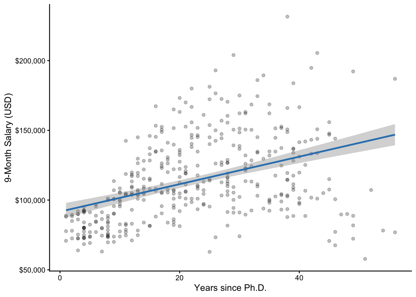
Figure 5.1: A scatterplot of years since Ph.D. and salary along with the line of best fit. The gray band represents the 95% confidence interval (CI).
Specifically, the simple linear regression is a specific case of ordinary least squares (OLS) regression. OLS is one of the several ways that we can calculate the error term.↩︎
\(m_{rank}=k_{rank}-1=3-1=2\)↩︎
yrs.since.phd: \[F = \frac{MSR}{MSE} = \frac{\frac{SSR}{df_R}}{\frac{SSE}{df_E}} = \frac{\frac{6.39e10}{1}}{\frac{2.99e11}{395}} = \frac{6.39e10}{7.58e8} = 84.23\]↩︎(Intercept): \[t = \frac{Estimate}{Std.\ Error} = \frac{91718.7}{2765.8} = 33.16\]↩︎(Intercept): \[t = \sqrt{F} = \sqrt{1099.71} = 33.16\]↩︎\[b_1 = \frac{\Delta Y}{\Delta X} = \frac{\Delta DV}{\Delta IV} = \frac{\Delta salary}{\Delta yrs.since.phd} = \frac{985.3}{1} = 985.3\]↩︎